- Published on
An introduction to Reinforcement Learning
- Authors
- Name
- Tan Ngoc Pham
- @ngctnnnn

Besides traditional data-based methods on Machine Learning, e.g. Clustering or Maximum Likelihood Estimation, Reinforcement Learning is a family in which tiny (or even no) data is required to do the training and testing phase. In this post, I would give a minor introduction on Reinforcement Learning, its basic concepts and methods.
Table of contents
1. What is Reinforcement Learning
Let say you want to help Pac-man on the game of Pac-man achieve the best score among different rounds and difficulties. However, you do not know surely how to play the game optimally and all you can do is to give Pac-man the instructions about the game only. On learning to find the best way to play the game with a maximum score, Pac-man has to play the game continuously, continuously, and continuously. That is the most basic understanding on what Reinforcement Learning looks like.

Mathematically, we could denote Pac-man as an agent and the game as the environment:
- One random strategy to play the Pac-man game as a policy (π ∈ Π).
- One position of Pac-man at a specific time as a state (s ∈ S).
- An event that Pac-man moves forward (or backward of left or right) as an action (a ∈ A).
- A score that Pac-man received after taking an action as the reward (r ∈ R).
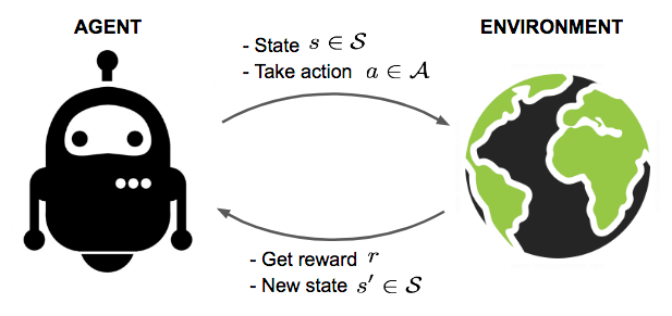 Fig 1. An illustration on Reinforcement Learning
The ultimate goal of Reinforcement Learning is to find an optimal policy π* which gives the agent a maximum reward r* on any diverse environments.
2. Principal (mathematical) concepts of Reinforcement Learning
a. Transition and Reward
Dummies' reinforcement learning algorithms often require a model for the agent to learn and infer. A model is a descriptor in which our agent would contact with the environment and receive respective solution feedbacks. Two most contributing factors to receive accurate feedbacks on how the agent performs are transition probability function (P) and reward function (R).
The transition probability function P, as it is called, records the probability of transitioning from state s to s’ after taking action and get a reward r at time t.
P(s', r | s, a) = p[St+1 = s', Rt+1 = r | St = s, At = a]
The equation could be understood as "the transition probability of state s to s' to get a reward r after taking action a equals to the conditional probability (p) of getting a reward of r after changing state from s to s' and taking an action a".
And the transition state function could be defined as:
Pss', a = P(s' |s, a) = ∑r ∈ R P(s', r | s, a)
The reward achieved on taking a new action a' is demonstrated using a reward function R and equals to the expected reward after taking an action a in the state s.
R(s, a) = 𝔼[Rt + 1 | St = s, At = a] = ∑r ∈ R(r) x ∑s' ∈ SP(s', r | s, a)
b. Policy
A policy π(·) is a mapping from a state s to its corresponding action a according to a specific strategy to take a suitable move toward the current state of our agent. A policy could be deterministic or stochastic, as which demonstrated:
- Stochastic policy: given a random state s, there is only one action a which always get the maximum reward r*.
π(s) = a
- Deterministic policy: given a random state s, the optimal action to get the highest reward is distributed over a probability distribution over all appropriate actions.
π(a | s) = Pπ[A = a | S = s]
c. State-Value and Action-Value Function
Value function, generally, is used as a metric to measure how good a state is and how high a reward we could achieve by staying in a state or taking an action.
Let denote G as the total reward that our agent would take, starting from time t:
Gt = Rt+1 + Rt+2 + ... = ∑k = 0 →∞(Rt + k + 1)
However, in reality, a reward would be more appetizing in the present than it is in the future (imagine which decision would you make if you are allowed to choose between receiving 100 bucks now or 100 bucks in 10 more years). It is, thus, a must to propose a coefficient of γ ∈ [0; 1] to penalize rewards in the future times. The above equation would be rewritten as follows
Gt = γRt+1 + γ2Rt+2 + ... = ∑k ∈ [0;∞)(γk Rt + k + 1)
Action-Value function
The Action-Value value (Q-value) is the expected total reward return of a state-action pair at a given time t and following policy π:
Qπ(s, a) = 𝔼π[Gt | St = s, At = a]
State-Value function
The State-Value value of a state s is the expected total reward return if we are in state s at time t
Vπ(s) = 𝔼π[Gt | St = s]
On stochastic policy, the relationship between Action-Value and State-Value is demonstrated as:
Vπ(s) = ∑a ∈ A [π(a | s) * Qπ(s, a)]
Qπ(s, a) = ∑s' ∈ S[P(s' | s, a) [R(s, a, s') + γVπ(s')]]
Optimal value and policy
By iterating around State-Value and Action-Value function, we could get the maximum return of the State-Value
V*(s) = maxπ{Vπ(s), Q*(s, a)} = maxπ[Qπ(s, a)]
The optimal policy would be the argmax from the optimal policy from the aforementioned maximum return of the State-Value
π* = argmaxπ{Vπ(s) π*}
3. A literature on preliminary approaches in Reinforcement Learning
In this section, I would drive you through the very initial solution for Reinforcement Learning
a. Dynamic Programming
Dynamic Programming is the first thought coming into Computer Scientists when Reinforcement Learning had just appeared as a successive of previous mathematics foundations such as Bellman Equations [Bellman (1959)] and Markov Decision Processes [Puterman (1994)]. There are a great number of DP-based and DP-inspired algorithms to deal with Reinforcement Learning. There lie two most highlighted algorithms when mentioned about DP in RL which are Policy Iteration and Value Iteration.
Both algorithms are DP algorithms based on Bellman Equations which aimed to find an optimal policy π* in a Reinforcement Learning environment using one-step look-ahead strategy.
| Policy Iteration | Value Iteration |
|---|---|
| Faster | Slower |
| Fewer iterations | More iterations |
| Guaranteed to converge | Guaranteed to converge |
| Algorithm is more sophisticated | Algorithm is more trouble-free |
| Start with a random policy | Start with a random value function |
| Cheaper computational costs | More expensive computational costs |
Table 1. A minor comparison between Policy Iteration and Value Iteration.
Policy Iteration
In policy iteration, one fixed policy is utilized firstly. Then, the algorithm would traverse through iterations, on every iteration, the policy is evaluated and updated gradually until the convergence.
def policy_iteration(env, max_iters, gamma):
    # Intialize a random policy
    policy = np.zeros(env.observation_space.n, dtype=np.int)
    for i in range(len(policy)):
        import random
        policy[i] = random.randint(0, 3)

    for i in range(max_iters):
        policy_stable = True

        # Evaluate the present policy
        v_values =  policy_evaluation(env,
                                      max_iters=max_iters,
                                      gamma=gamma,
                                      policy=policy)

        # Update the policy
        new_policy = policy_improvement(env,
                                        gamma=gamma,
                                        v_val=v_values,
                                        policy=policy)

        # Check convergence
        if np.all(np.array_equiv(policy, new_policy)):
            policy_stable = True
            print(f'Converged at {i}-th iteration')
            break
        else:
            policy_stable = False
        policy = new_policy.copy()
    return policy
Value Iteration
Value Iteration, on the other hand, begins with a selected value function and iterates over that value function. Value Iteration undergoes a heavier computing process by taking a maximum over the utility function for all possible actions. And subsequently, Value Iteration has a tendency to take more iterations before fully converged compared to the Policy one.
def value_iteration(env, max_iters, gamma):
    v_values = np.zeros(env.observation_space.n)

    for i in range(max_iters):
        prev_v_values = np.copy(v_values)

        # Compute the value for state
        for state in range(env.observation_space.n):
            q_values = []
            # Compute the q-value for each action
            for action in range(env.action_space.n):
                q_value = 0
                # Loop through each possible outcome
                for prob, next_state, reward, done in env.P[state][action]:
                    q_value += prob * (reward + gamma * prev_v_values[next_state])

                q_values.append(q_value)

            # Select the best action
            best_action = np.argmax(q_values)
            v_values[state] = q_values[best_action]

        # Check convergence
        if np.all(np.isclose(v_values, prev_v_values)):
            print(f'Converged at {i}-th iteration.')
            break

    return v_values
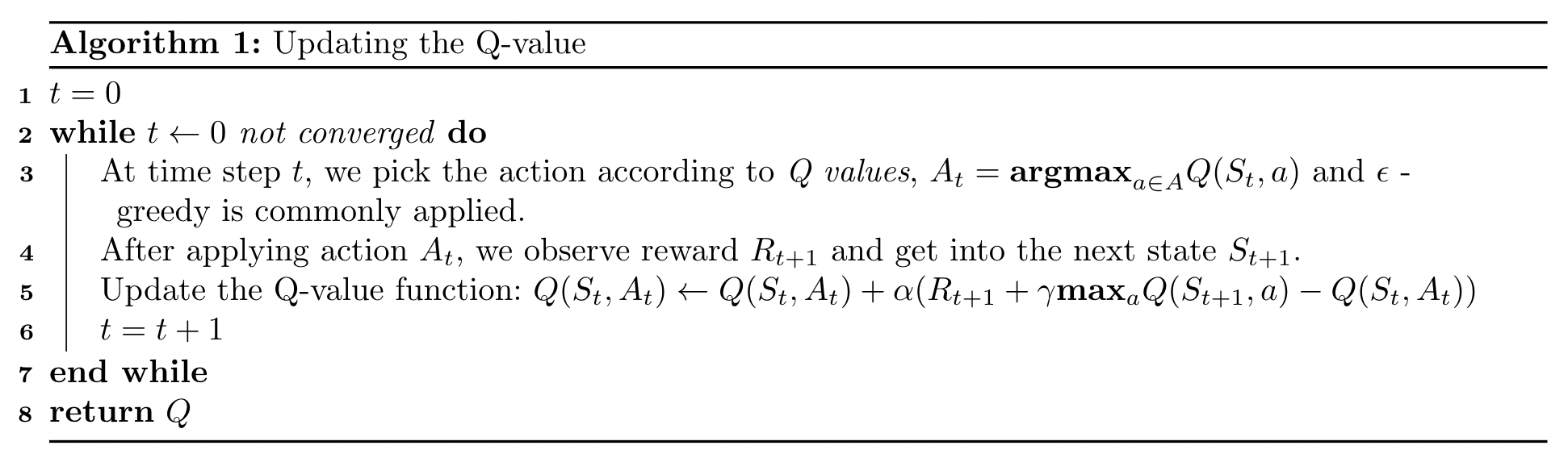
b. Q-Learning
Q-Learning is a model-free reinforcement learning algorithm to learn the quality of action a to tell the agent which actions to execute at a certain state s. It does not require a model of a certain environment. It can handle dynamically environmental problems and achieve rewards without any adaptations. The development of Q-Learning is actually a breakthrough in the early days of reinforcement learning.
The interesting point in Q-Learning is the independence of the current policy to choose the second action at+1. It, essentially, estimates Q* among the best Q-values, but it does not matter which action leads to this maximum Q-value and in the next step, this algorithm does not have to follow that policy.
4. Conclusions
- Throughout this blog, I have brought to you the most preliminary concepts on what Reinforcement Learning looks like, its mathematical fundamental and some of the algorithms to deal with Reinforcement Learning problems.
- Further construction in Reinforcement Learning and more intensive algorithms surrounding would be settled on later posts on this blog.