- Published on
Neural Architecture Search
- Authors
- Name
- Tan Ngoc Pham
- @ngctnnnn
The needs for appropriate deep neural networks for most modern problems have increased dramatically, and finding the right architecture is a challenge. Almost deep architectures nowadays are manually designed with tremendous times of trial-and-errors and state-of-the-arts are those with multiple layers, connections ignoring a suitable explanation.
Table of contents
1. Introduction
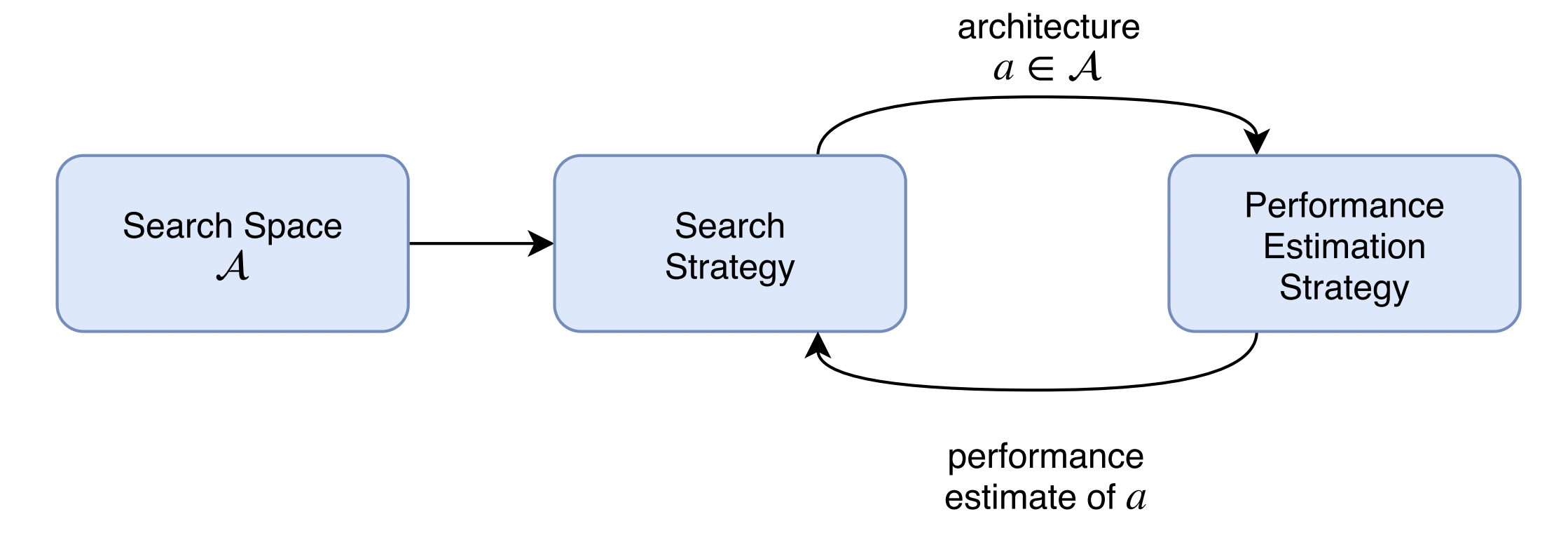
- NAS's concept begins with a search space of S, which could be under the form of different to-find-layers (macro-level), various operations (micro-level) or even different complete architectures that we would like to find. The paradigm then flows to the search strategy in which our heuristics would perform their strength towards the problem, e.g. Genetic Algorithm, Reinforcement Learning.
- On applying the suitable search strategy to the search space, one (or many) architectures is picked up from the search space and put into the evaluation step. The chosen architecture is evaluated by real training on the given dataset and the fitness is returned as the form of our wanted metric for the problem.
- This whole procedure is repeated continuously until we found out the outperformed architecture for the problem or the algorithm met the terminated criterion, i.e. number of iterations, out of computational resources.
 Fig 1. Paradigm of NAS
2. Recent literature on Neural Architecture Search
a. Neural Optimizer Search with Reinforcement Learning
Mentioning NAS often means mentioning the work of Zoph and Le. 2017 on first bringing out the concept of finding neural architecture and how to resolve the problem. The very first solution for the NAS is to use a Recurrent Neural Network controller to generate a string representating the outcome network using Reinforcement Learning in which:
- The environment for the NAS is the search space of the problem.
- The actions are the search strategies that we would love to apply on.
- The reward is the accuracy of the chosen architecture trained on CIFAR-10 dataset.
The results towards the initial approach is outstanding when the final architectures have a tendency to converge near the state-of-the-art architectures that we know nowadays, e.g. AlexNet [Krizhevsky et al. (2012)] or VGG [Simonyan and Zisserman (2014)]. And moreover, the result architecture is not overfitted on the train dataset but has a strong transferability when testing on different datasets.
However, the approach costs a fortune of computational resources since each step, they have to construct the network from the beginning and the network has to be trained from scratch. The power of the very first method of NAS and the limitations from computational process is the primary motivation for later works on various aspects which are search spaces, datasets, training-free methods and so on.
b. NAS Benchmark:
On resolving the problem of training from scratch on the way, NAS Benchmark has been born to minimize the computational costs that researchers demand when doing the NAS. There are a great amount of NAS Benchmarks nowadays but there are 2 most highlighted ones in the field.
- NAS-Bench-101 [Ying et al. (2019)]
Developed by Google, NAS-Bench-101 is constructed with a compact, yet expressive, search space, exploiting graph isomorphisms to identify 423 000 unique convolutional architectures on CIFAR-10 dataset. NAS-Bench-101 is simply used by querying based on the upper-triangular matrix representating the formulation of the network we would like to evaluate.
# Load the data from file (this will take some time)
nasbench = api.NASBench('/path/to/nasbench.tfrecord')

# Create an Inception-like module (5x5 convolution replaced with two 3x3
# convolutions).
model_spec = api.ModelSpec(
    # Adjacency matrix of the module
    matrix=[[0, 1, 1, 1, 0, 1, 0],    # input layer
            [0, 0, 0, 0, 0, 0, 1],    # 1x1 conv
            [0, 0, 0, 0, 0, 0, 1],    # 3x3 conv
            [0, 0, 0, 0, 1, 0, 0],    # 5x5 conv (replaced by two 3x3's)
            [0, 0, 0, 0, 0, 0, 1],    # 5x5 conv (replaced by two 3x3's)
            [0, 0, 0, 0, 0, 0, 1],    # 3x3 max-pool
            [0, 0, 0, 0, 0, 0, 0]],   # output layer
    # Operations at the vertices of the module, matches order of matrix
    ops=[INPUT, CONV1X1, CONV3X3, CONV3X3, CONV3X3, MAXPOOL3X3, OUTPUT])

# Query this model from dataset, returns a dictionary containing the metrics
# associated with this model.
data = nasbench.query(model_spec)
The result achieved on this benchmark is under the format of a json:
data = {
    'module_adjacency' : 0,
    'module_operations' : 0,
    'trainable_parameters' : 0,
    'training_time' : 0,
    'train_accuracy' : 0,
    'validation_accuracy' : 0,
    'test_accuracy' : 0
}
- NATS-Bench [Dong et al. (2021)]
The NATS-Bench is the upgraded version of a previous work NAS-Bench-201. NATS-Bench includes the search space of 15,625 neural cell candidates for architecture topology and 32,768 for architecture size on three dataset (CIFAR-10, CIFAR-100, ImageNet16-120).
"""
Create the benchmark instance
"""
from nats_bench import create
# Create the API instance for the size search space in NATS
api = create(None, 'sss', fast_mode=True, verbose=True)

# Create the API instance for the topology search space in NATS
api = create(None, 'tss', fast_mode=True, verbose=True)

"""
Query the performance
"""
# Query the loss / accuracy / time for 1234-th candidate architecture on CIFAR-10
# info is a dict, where you can easily figure out the meaning by key
info = api.get_more_info(1234, 'cifar10')

# Query the flops, params, latency. info is a dict.
info = api.get_cost_info(12, 'cifar10')
The result from querying NATS-Bench is a json of multiple metrics on 2 different epochs:
info = {
    'train-loss'     : 0,
    'train-accuracy' : 0,
    'train-per-time' : 0,
    'train-all-time' : 0,
    'test-loss'      : 0,
    'test-accuracy'  : 0,
    'test-per-time'  : 0,
    'test-all-time'  : 0
}
3. Conclusions
- Manual construction on deep neural networks is a time-consumed, high computational consuming and specified works.
- Neural Architecture Search is the field when we minimize the labour on evaluating separated architectures for a typical dataset.